Representation of a Three-Dimensional Moving Scene
Representation of a Three-Dimensional Moving Scene
Reference: An Invitation to 3-D vision, Chapter 2.
CheatSheet
| Rotation | Transformation | |
|---|---|---|
| vector form | $ w \in \mathbb{R}^3 $ | $ \xi = \begin{bmatrix} w & v \end{bmatrix}^T \in \mathbb{R}^6 $ : twist coordinates |
| exponential coordinates | $ \widehat{w} \in so(3) \subset \mathbb{R}^{3 \times 3} $ $ \widehat{w} \doteq \begin{bmatrix} 0 & -w_3 & w_2 \\ w_3 & 0 & -w_1 \\ -w_2 & w_1 & 0 \end{bmatrix} $ | $ \hat{\xi} \in se(3) \subset \mathbb{R}^{4 \times 4} $ : twist $ \widehat{\xi} \doteq \begin{bmatrix} \widehat{w} & v \\ 0 & 0 \end{bmatrix} $ |
| matrix form | $ R = e^{\hat{w}} \in SO(3) \subset \mathbb{R}^{3 \times 3} $ | $ T = e^{\hat{\xi}} \in SE(3) \subset \mathbb{R}^{4 \times 4} $ |
| exponential map | $ e^{\widehat{w}t} = I + \widehat{w}sin(t) + \widehat{w} ^2 (1-cos(t)) $ where $ \begin{Vmatrix} w \end{Vmatrix}=1 $ | $ e^{\widehat{\xi}t} = \begin{bmatrix} e^{\widehat{w}} & \left( I - e^{\widehat{w}} \right) \widehat{w} v + w \widehat{w}^T v \\ 0 & 1 \end{bmatrix} $ |
2.1 Three-dimensional Euclidean space
A point in the Euclidean space:
\[\mathbf{X} \doteq \begin{bmatrix} X_1 \\ X_2 \\ X_3 \end{bmatrix} \in \mathbb{R}^3, \mathbb{E}^3\]A vector in the Euclidean space
\[v \doteq \mathbf{Y - X} \in \mathbb{R}^3\]Inner product of two vectors:
\[\left\langle u,v \right\rangle \doteq u^Tv = u_1 v_1 + u_2 v_2 + u_3 v_3, \forall u,v \in \mathbb{R}^3\]Cross product of two vectors:
\[u \times v \doteq \begin{bmatrix} u_2v_3 - u_3v_2 \\ u_3v_1 - u_1v_3 \\ u_1v_2 - u_2v_1 \end{bmatrix} \in \mathbb{R}^3\]For fixed $ u $, the cross product can be represented by a map from $ \mathbb{R}^3 $ to $ \mathbb{R}^3: u \mapsto u \times v $. We define this mapping matrix by
\[\widehat{u} \doteq \begin{bmatrix} 0 & -u_3 & u_2 \\ u_3 & 0 & -u_1 \\ -u_2 & u_1 & 0 \end{bmatrix} \in \mathbb{R}^{3 \times 3}\]such that $ u \times v = \widehat{u}v $. Note that $ \widehat{u} $ is a skew-symmetric matrix, i.e. $ \widehat{u}^T = -\widehat{u} $.
The cross product defines a (one-to-one) map between a vector u and a $3 \times 3$ skew-symmetric matrix $ \widehat{u} $. The map is defined by a hat-operator
\[\wedge : \mathbb{R}^3 \rightarrow so(3); u \mapsto \widehat{u}.\]2.2 Rigid-body motion
Rigid-body: the distance between any pair of points $ (p,q) $ on it does not change over time as the object moves.
Euclidean transformation: a map that preserves the Euclidean distance between every pair of points. The set of all Euclidean transformation in 3-D space is denoted by $ E(3) $.
\[g: \mathbb{R}^3 \to \mathbb{R}^3; X \mapsto g(X)\]
Suppose a vector $ v=\mathbf{Y} - \mathbf{X} $. After the transformation of $g$, we obtain a new vector \(u = g_*(v) \doteq g(\mathbf{Y}) - g(\mathbf{X})\) where \(\begin{Vmatrix} g_*(v) \end{Vmatrix} = \begin{Vmatrix} v \end{Vmatrix}.\)
Some Euclidean transformations are not physically realizable. For example the map
\(f: \begin{bmatrix} X_1, X_2, X_3 \end{bmatrix} \mapsto \begin{bmatrix} X_1, X_2, -X_3 \end{bmatrix}\) preserves distances but not orientations. (reflection)
The map or transformation induced by a rigid-body motion is called a special Euclidean transformation. The word “special” indicates the fact that a transformation is orientation-preserving.
Rigid-body motion or special Euclidean transformation: A map that preserves the norm and the cross product of any two vectors
- norm: \(\begin{Vmatrix} g_*(v) \end{Vmatrix} = \begin{Vmatrix} v \end{Vmatrix}, \forall v \in \mathbb{R}^3\)
- cross product: \(g_*(u) \times g_*(v) = g_*(u \times v), \forall u, v \in \mathbb{R}^3\)
- (consequently) angle or inner product: \(\left\langle u,v \right\rangle = \left\langle g_*(u), g_*(v) \right\rangle\)
Let us define a Cartesian coordinate frame, with its principal axes given by three orthonormal vectors $ e_1, e_2, e_3 \in \mathbb{R}^3 $ ($e_1 \times e_2 = e_3 $, right-handed frame)
\[e_i^T e_j = \delta_{ij} \doteq \begin{cases} 1 & \mbox{if } i = j \\ 0 & \mbox{if } i \ne j \end{cases}\]After a rigid-body motion $ g $,
\[g_*(e_i)^T g_*(e_j) = \delta_{ij} , \quad g_*(e_1) \times g_*(e_2) = g_*(e_3)\]The resulting vectors still form a right-handed frame.
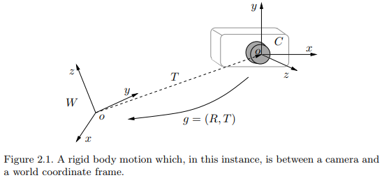
When a camera moves, the camera frame also moves along with the camera. The configuration of the camera is then determined by two components:
- Translational part $ T $ : the vector between the origin of the world frame and that of the camera frame.
- Rotational part $ R $ : the relative orientation of the camera frame $ C $, with coordinate axes $ (x,y,z) $, relative to the fixed world frame $ W $ with coordinate axes $ (X,Y,Z) $
2.3 Rotational motion and its representations
2.3.1 Orthogonal matrix representation of rotations
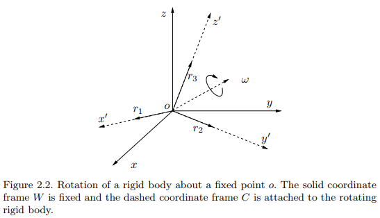
The frame C relative to the frame W is determined by the three orthonormal vectors:
\[r_1=g_*(e_1), r_2=g_*(e_2), r_3=g_*(e_3) \in \mathbb{R}^3.\]Then the configuration of the rotating object is determined by the $ 3 \times 3 $ matrix $ R_{wc} \doteq \begin{bmatrix} r_1, r_2, r_3 \end{bmatrix} \in \mathbb{R}^3 $
Since $ r_1, r_2, r_3 $ form an orthonormal frame,
\[\begin{align} & r_i^T r_j = \delta_{ij} \doteq \begin{cases} 1 & \mbox{if } i = j \\ 0 & \mbox{if } i \ne j \end{cases} \\\\ & R_{wc}^T R_{wc} = R_{wc} R_{wc}^T = I, \quad R_{wc}^{-1} = R_{wc}^T: \text{orthogonal matrix} \end{align}\]Since we only deal with a right-handed frame, $ det(R_{wc}) = +1 $. Hence $ R_{wc} $ is a special orthogonal matrix, which is denoted by
\[SO(3) \doteq \left\{ R \in \mathbb{R}^{3\times3} \middle|\ R^TR=I,\ det(R)=+1 \right\}\]
The space $ SO(3) $ is referred as the special orthogonal group of $ \mathbb{R}^3 $ or simply rotation group.
Suppose that for a given point $ p $, its coordinates in the world frame $ W $ is $ X_w = \left[ X_{1w}, X_{2w}, X_{3w} \right] $.
Since $ r_1, r_2, r_3 $ form a basis for $ \mathbb{R}^3 $, $ X_w $ can also be expressed as
\[X_w = X_{1c}r_1 + X_{2c}r_2 + X_{3c}r_3\]where $ X_c = \left[ X_{1c}, X_{2c}, X_{3c} \right] $ is the coordinates of the same point $ p $ in the frame $ C $ relative to the frame $ W $.
\[\begin{aligned} & X_w = X_{1c}r_1 + X_{2c}r_2 + X_{3c}r_3 = R_{wc}X_c \\\\ & X_c = R^{-1}_{wc}X_w = R^T_{wc}X_w \end{aligned}\]$ R_{wc} $ transforms the coordinates $ X_c $ in the frame $ C $ to its coordinates $ X_w $ in the frame $ W $
2.3.2 Canonical exponential coordinates for rotations
Given a trajectory $ R(t) $ that describes a continuous rotational motion, the rotation must satisfy $ R(t)^TR(t) = I$.
By computing the derivative with respect to time $ t $,
\[\dot{R} R^T(t) + R(t) \dot{R}^T(t) = 0 \quad \Rightarrow \quad \dot{R}(t) R^T(t) = -(\dot{R}(t) R^T(t))^T\]The resulting equation shows that $ \dot{R}(t) R^T(t) \in \mathbb{R}^{3 \times 3} $ is a skew-symmetric matrix. There must exist a vector $ w(t) \in \mathbb{R}^3 $ such that
\[\begin{aligned} & \dot{R}(t) R^T(t) = \widehat{w}(t) \\\\ & \dot{R}(t) = \widehat{w}(t) R(t) \end{aligned}\]The space of all skew-symmetric matrices is denoted by
\[so(3) \doteq \left\{ \widehat{w} \in \mathbb{R}^{3 \times 3} \mid w\in \mathbb{R}^3 \right\}.\]
Note that $ so(3) $ depends only on three parameters.
Since the above equation is a linear ordinary differential equation (ODE), $ R(t) $ can be interpreted as the state transition matrix. Assuming $ R(0) = I $, the solution is
\[\begin{align} & R(t) = e^{\widehat{w}t} \\\\ & \text{where } e^{\widehat{w}t} \text{ is the matrix exponential} \\\\ & e^{\widehat{w}t} = I + \widehat{w}t + {(\widehat{w}t)^2 \over 2!} + \cdots + {(\widehat{w}t)^n \over n!} + \cdots \end{align}\]The matrix exponential indeed defines a map from the space $ so(3) $ to $ SO(3) $, the so-called exponential map
\[exp: so(3) \to SO(3); \quad \widehat{w} \mapsto e^{\widehat{w}}\]
We can verify the matrix $ e^{\widehat{w}t} $ is a rotation matrix.
\[\left( e^{\widehat{w}t} \right)^{-1} = e^{-\widehat{w}t} = e^{\widehat{w}^Tt} = \left( e^{\widehat{w}t} \right)^T\]Hence $ \left( e^{\widehat{w}t} \right)^T e^{\widehat{w}t} = I $.
The physical interpretation of $ R(t) = e^{\widehat{w}t} $ is that if $ \begin{Vmatrix} w \end{Vmatrix} = 1 $, $ R(t) = e^{\widehat{w}t} $ is simply a rotation around the axis $ w \in \mathbb{R}^3 $ by an angle $ t $ radians.
Theorem 2.8 (Logarithm of $ SO(3) $). For any $ R \in SO(3) $, there exists a (not necessarily unique) $ w \in \mathbb{R}^3 $ such that $ R = exp( \widehat{w} ) $. We denote the inverse of the exponential map by $ \widehat{w} = log(R) $.
Theorem 2.9 (Rodrigues’ formula for a rotation matrix). Given $ w \in \mathbb{R}^3$, the matrix exponential $ R = e^{\widehat{w}} $ is given by
\[e^{\widehat{w}} = I + {\widehat{w} \over \begin{Vmatrix} w \end{Vmatrix}} sin(\begin{Vmatrix} w \end{Vmatrix}) + {\widehat{w}^2 \over \begin{Vmatrix} w \end{Vmatrix}^2} (1 - cos(\begin{Vmatrix} w \end{Vmatrix})\]
if $ \begin{Vmatrix} w \end{Vmatrix} = 1 $, $ {\widehat{w} \over \begin{Vmatrix} w \end{Vmatrix}} = \widehat{w}, \begin{Vmatrix} wt \end{Vmatrix} = t $, so that
\[e^{\widehat{w}t} = I + \widehat{w}sin(t) + \widehat{w} ^2 (1-cos(t))\]Note that the exponential map is not commutative.
\[e^{\widehat{w}_1} e^{\widehat{w}_2} \neq e^{\widehat{w}_2} e^{\widehat{w}_1} \neq e^{\widehat{w}_1 + \widehat{w}_2}\]2.4 Rigid-body motion and its representations
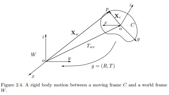
The figure illustrates a moving rigid object with a coordinate frame $ C $. The coordinates of the point $ p $ is either $ X_w $ in the world frame or $ X_c $ in the object frame. The relationship between them is given by
\[X_w = R_{wc}X_c + T_{wc}\]where $ R_{wc} \in SO(3) $ is the relative rotation between two frames and $ T_{wc} \in \mathbb{R}^3 $. The vector from the origin of the frame $ C $ to the point $ p $ in the world frame $ W $ is $ R_{wc}X_c $.
We denote the full rigid-body motion by $ g_{wc} = \left( R_{wc}, T_{wc} \right ) $, or simply $ g = \left( R, T \right ) $. In compact form, we rewrite
\[X_w = g_{wc}\left( X_c \right)\]The set of all possible configurations of a rigid body can then be described by the space of rigid-body motions or special Euclidean transformations
\[SE(3) \doteq \left\{ g = (R, T) \mid R \in SO(3), T \in \mathbb{R}^3 \right\}\]
2.4.1 Homogeneous representation
Rigid body motion, \( X_w = R_{wc}X_c + T_{wc} \), is not linear but affine. An affine transformation can be converted to linear on by homogeneous coordinates. In homogeneous coordinates, a point $ p \in \mathbb{R}^3 $ and a vector $ v \in \mathbb{R}^3 $ are represented as
\[\begin{aligned} & \bar{X} \doteq \begin{bmatrix} \mathbf{X} \\ 1 \end{bmatrix} \in \mathbb{R}^4 \\\\ & \bar{v} \doteq \begin{bmatrix} v \\ 0 \end{bmatrix} = \begin{bmatrix} \mathbf{X}(p) \\ 1 \end{bmatrix} - \begin{bmatrix} \mathbf{X}(q) \\ 1 \end{bmatrix} = \begin{bmatrix} v_1 \\ v_2 \\ v_3 \\ 0 \end{bmatrix} \in \mathbb{R}^4 \end{aligned}\]Using the homogeneous notation, the rigid-body motion can then be rewritten in a linear form.
\[\bar{X}_w = \begin{bmatrix} X_w \\ 1 \end{bmatrix} = \begin{bmatrix} R_{wc} & T_{wc} \\ 0 & 1 \end{bmatrix} \begin{bmatrix} \mathbf{X}_c \\ 1 \end{bmatrix} \doteq \bar{g}_{wc} \bar{X}_c\]$ \bar{g}_{wc} \in \mathbb{R}^{4 \times 4} $ is called the homogeneous representation of the rigid-body motion $ g_{wc} = \left( R_{wc}, T_{wc} \right) \in SE(3) $.
We can represent a rigid-body transformation of coordinates by a linear matrix multiplication. A matrix representation of the special Euclidean transformation is given by
\[SE(3) \doteq \left\{ \bar{g} = \begin{bmatrix} R & T \\ 0 & 1 \end{bmatrix} \middle| R \in SO(3), T \in \mathbb{R}^3 \right\} \in \mathbb{R}^{4 \times 4}\]
From the above definition, $ SE(3) $ forms a group.
\[\begin{align} & \forall g_1, g_2, g \in SE(3), \\\\ & \bar{g}_1 \bar{g}_2 = \begin{bmatrix} R_1 & T_1 \\ 0 & 1 \end{bmatrix} \begin{bmatrix} R_2 & T_2 \\ 0 & 1 \end{bmatrix} = \begin{bmatrix} R_1R_2 & R_1T_2 + T_1 \\ 0 & 1 \end{bmatrix} \in SE(3) \\\\ & \bar{g}^{-1} = \begin{bmatrix} R & T \\ 0 & 1 \end{bmatrix}^{-1} = \begin{bmatrix} R^T & -R^T T \\ 0 & 1 \end{bmatrix} \end{align}\]Note that rigid motions act differently on points (rotation and translation) and vectors (only rotation)
\[\begin{align} & \bar{g}(\bar{\mathbf{X}}) = \bar{g} \begin{bmatrix} \mathbf{X} \\ 1 \end{bmatrix} = R\mathbf{X} + T \\\\ & \bar{g}(v) = \bar{g} \begin{bmatrix} v \\ 0 \end{bmatrix} = Rv \end{align}\]2.4.2 Canonical exponential coordinates for rigid-body motions
From now on, for simplicity let us omit “-“ to indicate homogeneous representation and simply use $ g $.
Consider a moving rigid body described by $ SE(3): g(t) = \left( R(t), T(t) \right) $ or in the homogeneous representation
\[\begin{align} & g(t) = \begin{bmatrix} R(t) & T(t) \\ 0 & 1 \end{bmatrix} \in \mathbb{R}^{4 \times 4} \\\\ & \dot{g}(t) g^{-1}(t) = \begin{bmatrix} \dot{R}(t) & \dot{T}(t) \\ 0 & 1 \end{bmatrix} \begin{bmatrix} R(t)^T & -R(t)^T T(t) \\ 0 & 1 \end{bmatrix} \\\\ & = \begin{bmatrix} \dot{R}(t) R^T(t) & \dot{T}(t) - \dot{R}(t) R^T(t) T(t) \\ 0 & 1 \end{bmatrix} \in \mathbb{R}^{4 \times 4} \end{align}\]We know that $ \dot{R}(t) R^T(t) $ is a skew-symmetric matrix: there exists $ \widehat{w}(t) \in so(3) $ such that $ \widehat{w} = \dot{R}(t) R^T(t) $.
By defining a vector $ v(t) = \dot{T} - \widehat{w}(t)T(t) $, the above equation becomes a matrix, called a twist,
\[\widehat{\xi}(t) = \dot{g}(t) g^{-1}(t) = \begin{bmatrix} \widehat{w}(t) & v(t) \\ 0 & 0 \end{bmatrix} \in \mathbb{R}^{4 \times 4}\]Then we have \(\dot{g}(t) = \dot{g}(t) g^{-1}(t) g(t) = \widehat{\xi}(t) g(t)\).
The set of all twists is denoted by
\[se(3) \doteq \left\{ \widehat{\xi} = \begin{bmatrix} \widehat{w} & v \\ 0 & 0 \end{bmatrix} \middle|\ \widehat{w} \in so(3), v \in \mathbb{R}^3 \right\} \subset \mathbb{R}^{4 \times 4}\]
We also define two operators, $\wedge$ and $\vee$, to convert between a twist $ \widehat{\xi} \in se(3) $ and its twist coordinates $ \xi \in \mathbb{R}^6 $ as follows:
\[\begin{align} & \begin{bmatrix} \widehat{w} & v \\ 0 & 0 \end{bmatrix}^{\vee} \doteq \begin{bmatrix} w \\ v \end{bmatrix} \in \mathbb{R}^6 \\\\ & \begin{bmatrix} w \\ v \end{bmatrix}^{\wedge} \doteq \begin{bmatrix} \widehat{w} & v \\ 0 & 0 \end{bmatrix} \in \mathbb{R}^{4 \times 4} \end{align}\]Consider a case that $ \widehat{\xi} $ is a constant matrix: \(\dot{g}(t) = \widehat{\xi} g(t)\). This is a time-invariant linear ordinary differential equation. Assuming $ g(0) = I $, the solution is
\[\begin{align} & g(t) = e^{\widehat{\xi}t} \\\\ & \text{where the twist exponential is} \\\\ & e^{\widehat{\xi}t} = I + \widehat{\xi}t + {(\widehat{\xi}t)^2 \over 2!} + \cdots + {(\widehat{\xi}t)^n \over n!} + \cdots \end{align}\]By Rodrigues’ formula and properties of matrix exponential,
\[e^{\widehat{\xi}t} = \begin{bmatrix} e^{\widehat{w}} & \left( I - e^{\widehat{w}} \right) \widehat{w} v + w \widehat{w}^T v \\ 0 & 1 \end{bmatrix} = \begin{bmatrix} R & T \\ 0 & 1 \end{bmatrix} , \text{ if }\ w \neq 0.\]The exponential map defines a transformation from the space $se(3)$ to $SE(3)$,
\[exp: se(3) \to SE(3); \quad \widehat{\xi} \mapsto e^{\widehat{\xi}t}\]The twist $ \widehat{\xi} \in se(3) $ is also called the exponential coordinates for $SE(3)$
Theorem 2.11 (Logarithm of $SE(3)$). For any $ g \in SE(3) $, there exist (not necessarily unique) twist coordinates $ \xi \in (v, w) $ such that $ g = exp(\hat{\xi}) $. We denote the inverse to the exponential map by $ \hat{\xi} = log(g) $